CQF · EXAM 2 · QUANTITATIVE FINANCE

Monte CarloOption Pricing

European & Binary Calls under the Risk-Neutral Measure

A Monte Carlo pricing framework comparingEuler-Maruyama, Milstein and Black-Scholesacross European and binary call options.

The project examines risk-neutral pricing, stochastic discretisation, parameter sensitivity, numerical error, convergence and antithetic variates through a Python-based simulation framework.

50,000

Main simulation paths

252

Steps per year

Option types

Parameter sensitivities

PRICING FRAMEWORK

Problem & Methodology

Objective

Price European and binary call options as discounted risk-neutral expectations and benchmark the numerical estimates against closed-form Black-Scholes values.

V_t = e^−r(T−t)E^Q[Π(S_T)]

Payoffs

European Call
max(S_T − K, 0)

Binary Call
1_{S_T > K}

Black-Scholes

Closed-form benchmark used to assess pricing accuracy across every scenario.

Euler-Maruyama

First-order stochastic time discretisation of geometric Brownian motion.

Milstein

Higher-order discretisation incorporating the diffusion derivative correction term.

Antithetic Variates

Paired shocks Z and −Z used to investigate variance reduction and estimator efficiency.

IMPLEMENTATION

Simulation Design

S₀100

Underlying spot

K100

Strike

T1 year

Time to expiry

σ20%

Volatility

r5%

Risk-free rate

Market Parameters

↓

Risk-Neutral GBM

↓

Euler-Maruyama

Milstein

↓

European / Binary Payoffs

↓

Discounted Expected Payoff

↓

Black-Scholes Benchmark

↓

Error & Convergence Analysis

SENSITIVITY ANALYSIS

Parameter Space

S₀60 → 160

Underlying spot

K85 → 110

Strike

T1 day → 2 years

Maturity

σ10% → 35%

Volatility

r3% → 7%

Risk-free rate

NUMERICAL RESULTS

Key Results

BLACK-SCHOLES · BASE CASE

European Call

10.450584

BLACK-SCHOLES · BASE CASE

Binary Call

0.532325

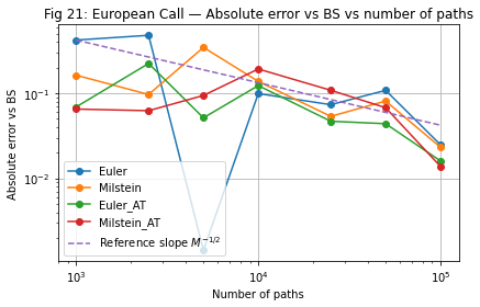
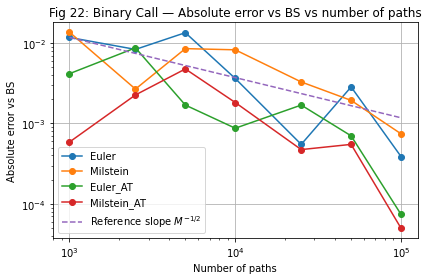
Payoff structure was the dominant driver of Monte Carlo error, with European calls exhibiting materially greater payoff dispersion than binary calls.

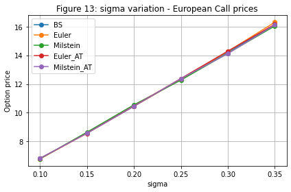
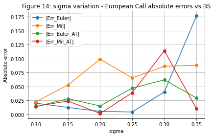
Euler and Milstein produced broadly similar pricing accuracy, with sampling variability often dominating discretisation differences.

Higher volatility and longer maturity increased numerical difficulty by widening the terminal payoff distribution.

Monte Carlo standard errors declined with the expected M^−1/2 convergence rate as the number of paths increased.

VISUAL ANALYSIS

Sensitivity & Convergence

European call prices as volatility varies — **Volatility sensitivity**European call estimates across Black-Scholes, Euler, Milstein and antithetic variants.

European call absolute pricing errors as volatility varies — **Numerical error under volatility variation**Absolute pricing error rises as payoff dispersion increases.

European call Monte Carlo price convergence — **European call convergence**Estimates stabilise around the Black-Scholes benchmark as the simulation count increases.

Binary call Monte Carlo price convergence — **Binary call convergence**The bounded payoff produces comparatively stable estimates.

European call standard error convergence — **European call standard error**Standard error follows the expected inverse square-root relationship with simulation size.

Binary call standard error convergence — **Binary call standard error**Convergence behaviour remains consistent with Monte Carlo theory.

PYTHON

Selected Implementation

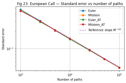
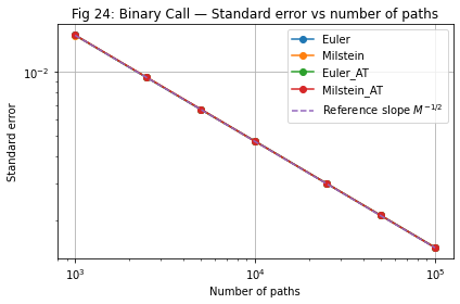
The project was implemented in Python with reusable functions for Black-Scholes pricing, stochastic simulation, payoff generation, sensitivity analysis and convergence testing.

Monte Carlo mean & standard errorPython

def mc_mean_se(samples: np.ndarray) -> Tuple[float, float]:
    samples = np.asarray(samples, dtype=float)

    return (
        float(samples.mean()),
        float(samples.std(ddof=1) / np.sqrt(samples.size))
    )

Milstein path updatePython

dW = sqrtdt * z[:, j]
corr = 0.5 * sigma**2 * (dW**2 - dt)

s *= (
    1.0
    + r * dt
    + sigma * dW
    + corr
)

PROJECT TAKEAWAY

What the Study Shows

The simulation framework reproduced the expected risk-neutral pricing behaviour and demonstrated that practical Monte Carlo accuracy was driven primarily by payoff dispersion and sampling variability. The project also showed that the theoretical higher-order accuracy of Milstein did not automatically translate into a material option-pricing advantage when compared with Euler at daily time steps.

PythonNumPyPandasSciPyMatplotlibMonte CarloBlack-ScholesStochastic Calculus